15 Sep How to set up Repeated-Measures Regressions in R

We analyze within-subjects designs with repeated-measures regressions, aka random-effects models. Learn how to set up such models in R. This concerns analyzing data with grouping, clustering, aka. hierarchical data, data with correlated errors, or data with violations of sphericity.

The names given to the models vary: multilevel model, random-effects model, longitudinal models, repeated-measures model, hierarchical models, they belong to linear mixed-effects models (LMEM), general linear model (GLM). I will use repeated-measures models.

Brief Reminder: Repeated-Measures Models

If you just want the R-code, skip this go directly to the R-code.

Repeated-measures data involves multiple data points from each participant, for example asking one question twice, or manipulating within-subject conditions – anything with more than one data point from a source or a group. Random effects models may be the term you’ve heard of in this case.

My toy use case: each participant answers four questions, like “How much do you like snack 0, 1, 2, 3”?

In simplified terms, our regression models should allow that participant A answers the four questions in her own idiosyncratic manner, and participant B answers them in his own special manner, causing the data from participant A to be similar to themselves, and the data of B to be similar to themselves. That’s a simplification, but suffices. A Frontier’s article (Magezi, 2015) nicely details these regressions, for your deeper understanding. These models are sometimes called linear random-effects models, but this terminology is not universal.

Setting up Repeated-Measures Regression Models

For those wanting to replicate this exactly, get the sample_data.csv on github. The simulated data has N=3, each answered four questions q0, q1, q2, q3.

[code lang=”R”]simple.df <- read.csv2(“test_data.csv”)
head(simple.df)
# participant age question answer
# 1 p1 38 0 7.554094
# 2 p1 38 1 17.305572
# 3 p1 38 2 28.220654
# 4 p1 38 3 36.481638
# 5 p2 21 0 3.642820
# 6 p2 21 1 9.782579
.
.
.[/code]

Standard regression (not a repeated-measures model)

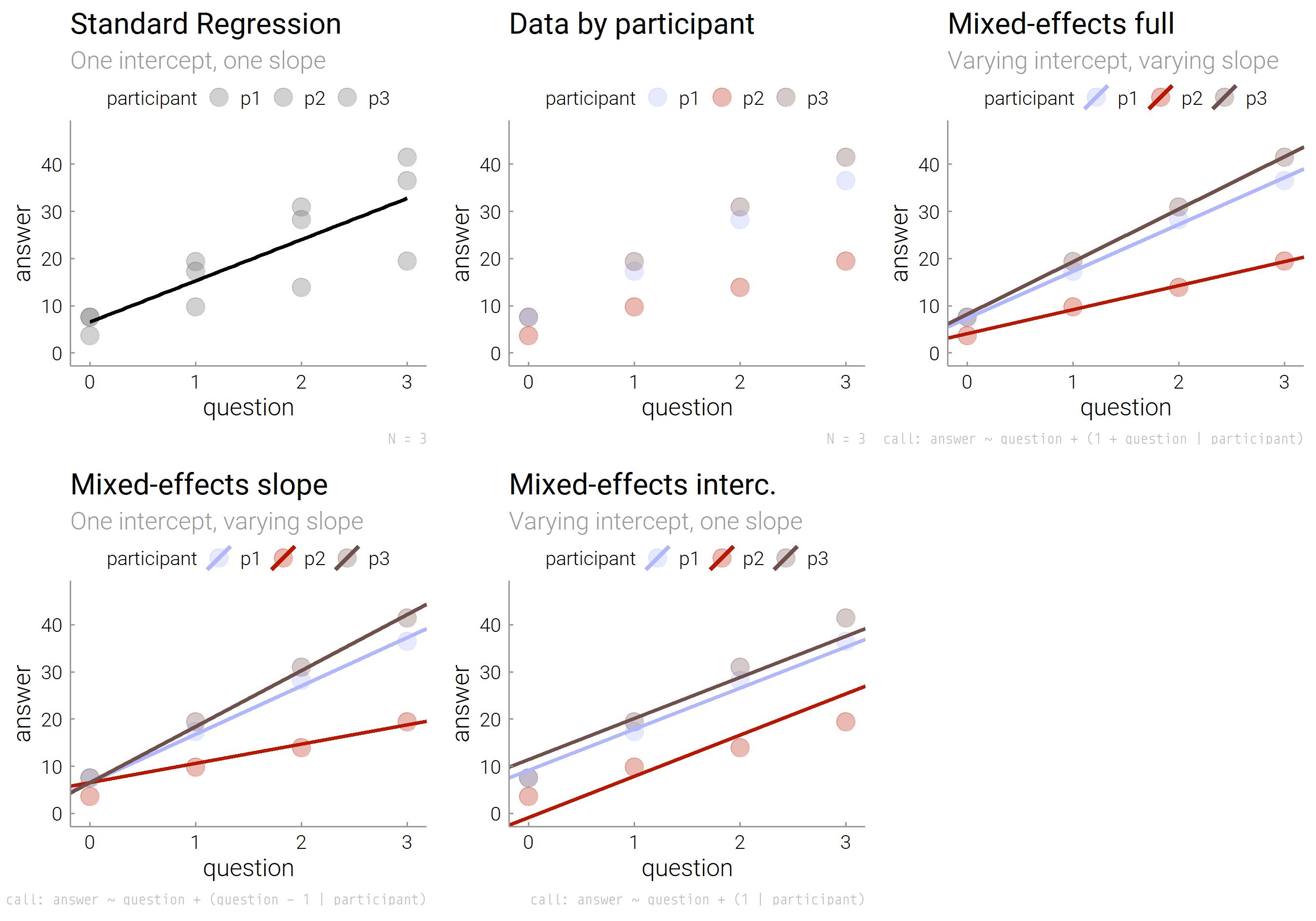
Let’s start with a standard regression, regressing variables answer on question, lm(answer ~ question, data = simple.df) is shown in the left plot, it looks ok. However, coloring the raw data by participant, we see clusters in the right plot. The grey participant p3 increases her answers to questions 0-3 much more than the red participant p2. That’s clustering of the answer variable within the participant variable.

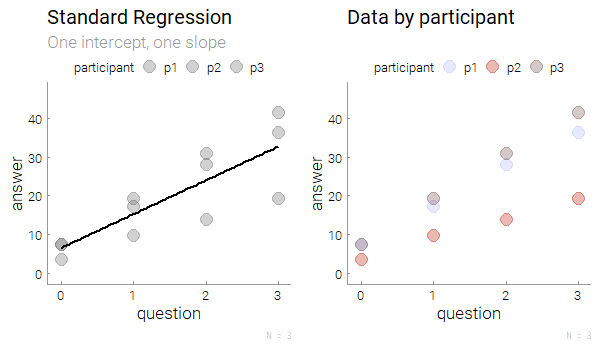
What’s important is that the standard regression knows no clusters. It always assumes that one intercept and one slope fits them all. This is an assumption we can relax. Let’s run regressions, that can model the fact that answers by different people differ in slopes and intercepts. You need the lme4 package:

[code lang=”R”]library(lme4) # if package doesn’t exist: install.packages(“lme4”)[/code]

To take your grouped/repeated data into account, you have to tell the model to cluster data within each participant or whatever your grouping variable is.

1. Intercepts varying per group

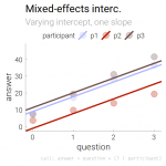The first regression, which accounts for grouping/repeated measures, models different intercepts but assumes one slope to fit them all. The plot shows different heights of the fitted lines per participant, but lines are parallel with common slopes. To this end, add + (1 | participant) to the regression formula:

[code lang=”R”]lmer(answer ~ question + (1 | participant), data=simple.df)[/code]

2. Slopes varying per group

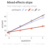The second regression, which accounts for grouping/repeated measures, allows just different slopes while assuming one intercept to fit them all. The graph illustrates how only the slope of the fitted lines vary by person, but all lines have the same height at zero, having identical intercepts. To this end, add + (question - 1 | participant) to the regression formula:

[code lang=”R”]lmer(answer ~ question + (question – 1 | participant), data=simple.df)[/code]

3. Slopes and intercepts varying per group

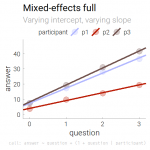The last regression, which accounts for grouping/repeated measures, allows both intercepts and slopes to differ between participants. The graph illustrates how both the slopes and the heights of the fitted lines vary. To this end, add + (1 + question | participant) to the regression formula:

[code lang=”R”]lmer(answer ~ question + (1 + question | participant), data=simple.df)[/code]

You can also add other predictors, like age.

[code lang=”R”]lmer(answer ~ age + question + (1 + question | participant), data=simple.df)[/code]

Then the model is sometimes called a mixed model, but John Salvatier, quoting Andrew Gelman, points out here, the name random effects, and fixed effects are not universally well-defined.

Compare fit of regressions

Store regression models
[code lang=”R”]model_in <- lmer(answer ~ question + (1 | participant), data=simple.df)
model_sl <- lmer(answer ~ question + (question – 1 | participant), data=simple.df)
model_in_sl <- lmer(answer ~ question + (1 + question | participant), data=simple.df)
[/code]

Compare models with anova():

[code lang=”R”]library(lmerTest)
anova(model_in, model_sl, model_in_sl)[/code]

A table with model fit indices results.

Report regressions with varying terms

Clarify whether your model in detail (more is less, use footnotes if you must).  “Keep it maximal” is the title of a paper advising to report the co-variance structure in the appendix (Barr, Levy, Scheepers, & Tily, 2013). Do not say “a random effects model showed, …”, you could mean “model with variying intercept”, or “model with varying slope” or both. Report exactly what you did, enable others to repeat your analysis. The parameters that can vary are often called ‘random effects’. Report as recommended (Hesser, 2015; Jackson, 2010), like so:

Report verbally, including the software, e.g. model 3

A linear regression (using lme4 in R) with random participant slope and intercept revealed that _ increased with _.

Alternatively, report the model equation, e.g. model 3

A random effects regression ([latex]answer_{ij} = \beta_0 + p_{0i} + (\beta_1 + q_{1j}) q_j + \epsilon_{ij}[/latex]) showed that _ increased with _.

A translation of your R-code to the equation is in Table 1 (Barr et al., 2013).

Some like to report with R-syntax, and I think I did it once, too, like in “A random effects regression (answer ~ question + (1 + question | participant) showed …”, but this could disadvantage SAS, Matlab, python, etc. users.