
20 Aug Optimization via ML and SSE for Myung (2003)
R script implementing the tutorial on maximum likelihood estimation in Myung (2003). It optimizes a parametrized retention function via maximum likelihood and the sum of squared errors.
Retention function?
Retention functions model recalling things becomes worse as time passes. Retention functions need to be some decreasing function of time, predicting the probability of correct recall. Many functional forms are used in the literature. Two thereof are a power law and an exponential decay function.
Let $latex t$ denote the time passed until recall. Let $latex x,y $ be the two free parameters.
The power law retention model is
$latex \hat{p} = x t^{-y} $
,
whereas the exponential retention model is
$latex \hat{p} = x \exp(-yt) $
Goal of optmizing
We want to obtain values for the free parameters $latex x$ and $latex y$, seperately for each model. Given real data of people recalling things at different time points – which parameter values $latex x^*,y^* $ bring the predicted retention probability closest to the real data? The star ($latex ^*$) is commonly used to denote these very values yielding the best fit of predictions to data. Myung provides a nice introduction explaining that “close to the data” can be calculated by different measures of fit such as maximum likelihood and the sum of squared errors.
Step 1: Write afit function
The fit function returns one number. That is, the fit of model predictions to data. Our function first predicts retention probabilities from the model, and then computes the fit to the observed data.
Our fit function will take as additional argument the model we want to fit. Important, writing this function we want one argument with the two model prameter. This becomes important for the optimization.
[code lang=”R”]
fitfun = function(f, p, n, t, model, costfn) {
# f: free parameter for the retention models [vector]
# p: observed recall probabilities for times t [vector]
# n: observed number of people [scalar]
# t: observed times of the observations [scalar]
# model: which model to use [string]
# costfn: which fit measure to use [string]
if(length(f) != 2) { # Check
stop(“Argument x must be of length 2, but is: “, paste(x), “.”)
}
x = f[1] #par: decay rate
y = f[2] #par: connection strength
n1 = p * n #data: number of responses “1”
n2 = (1-p) * n #data: number of responses “0”
e = 10^-6 #epsilon: we’ll use it for p_hat if p_hat=0 in the loglik to avoid log(0) = -Inf
# Predictions
if ( model==”power” ) {#Power law model
p_hat = x * t^(-y)
} else if ( model==”exponential” ) { #Exponential law model
p_hat = x * exp(-y * t)
}
# Fits
if(costfn == “SSE”) { #Sum of sq. errors
SSE = sum((p – p_hat)^2)
return(SSE)
} else if (costfn==”logLik”){ #Sum of log likelihood
p_hat = ifelse(p_hat==0,e, ifelse(p_hat==1,(1-e), p_hat)) #Ensure 0 < p_hat < 1
logLik = n1 %*% log(p_hat) + n2 %*% log(1-p_hat) #Log likelihood
return(-1 * logLik) #scale to get minimization problem
}
}
[/code]
Step 2: optimize this fit function’s value
We want to find the best-fitting values of x. In our case, we want to minimize the fit value over x. Therefore we will vary x and keep all other parameter constant. The next code optimizes our fit function given a fixed set of observations (fixed p, n), one model (fixed model) and one fit measure (fixed costfn).
Let’s first generate observed retention data.
[code lang = “R”]# Observed data
obs_p = c(.94, .77, .40, .26, .26, .16) #retention probabilities
obs_n = 100 #number of people
obs_t = c(1, 3, 6, 9, 12, 18) #points in time[/code]
The optimization itself will be carried out by the optim function from the neldermead package as follows: We first choose random parameter values $latex x, y$ from which the optimization starts. Further we chose a lower and upper bound on $latex x, y$ such that they stay between 0 and 1.
[code lang = “R”]set.seed(458)
# Initialize parameter
init_par = runif(2) #starting values for the parameter
low_par = c(0,0) #bounds for constr. optimization
up_par = c(1,1)
[/code]
Thereafter, the optim function runs the optimization for us. In this example we tell the fit function to use exponential model as model and log likelihood as fit function. Note, that for optim to work, the free parameters (the parameters to optimize) must be the first argument of the fit function.
[code lang = “R”]
library(“neldermead”) #for optimization
set.seed(458) #replicability
optim(
par = init_par, #Parameter starting values
fn = fitfun, #fit function
p = pobs, #arguments to fit_M()
n = nobs, # -“-
t = tobs, # -“-
model = “exponential”, # -“-
costfn = “logLik”, # -“-
method = “L-BFGS-B”, #algorithm, see see http://127.0.0.1:23627/library/stats/html/optim.html
lower = low_par, #bounds
upper = up_par
)
[/code]
Step 3: Optimize it
The above code answers the question which parameter values we should chose for the exponential model if we optimize the log likelihood. But we want to get this for the exponential and the power law model and for the log likelihood and the sum of squared errors. Therefore we repeat the optimization for all models and all fit measures. We store the models in a vector that holds the model names and loop through that vector. The same for the costfunctions.
[code lang = “R”]
library(“neldermead”) #for optimization
set.seed(458) #replicability
Models = c(“power”,”exponential”) #Holds model names
Costfuns = c(“logLik”,”SSE”) #Holds cost function names
# For each costfunction, and each model: do the fit
for (i_c in 1:length(Costfuns)) {
for (i_m in 1:length(Models)){
# store results in Xstar
Xstar = optim(
par = init_par, #Parameter starting values
fn = fitfun, #fit function
p = pobs, #arguments to fit_M()
n = nobs, # -“-
t = tobs, # -“-
model = Models[i_m], # -“-
costfn = Costfuns[i_c], # -“-
method = “L-BFGS-B”, #algorithm, see see http://127.0.0.1:23627/library/stats/html/optim.html
lower = low_par, #bounds
upper = up_par
)
}
}
[/code]
Further we would like to have the results in one table. Thus we write a data.frame R to hold the results.
[code lang = “R”]
library(“neldermead”) #for optimization
set.seed(457) #replicability
Models = c(“power”,”exponential”) #Holds model names
Costfuns = c(“logLik”,”SSE”) #Holds cost function names
R = data.frame(logLik_power=rep(0,3),logLik_exponential=0,SSE_power=0,SSE_exponential=0,row.names=list(“Fit”,”x”,”y”)) #Initiate results data frame
# Simulate for all Costfuns x Models and write it in corresponding column of R
for (i_c in 1:length(Costfuns)) {
for (i_m in 1:length(Models)){
# store results in Xstar
Xstar = optim(
par = init_par, #Parameter starting values
fn = fitfun, #fit function
p = pobs, #arguments to fit_M()
n = nobs, # -“-
t = tobs, # -“-
model = Models[i_m], # -“-
costfn = Costfuns[i_c], # -“-
method = “L-BFGS-B”, #algorithm, see see http://127.0.0.1:23627/library/stats/html/optim.html
lower = low_par, #bounds
upper = up_par
)
colname = paste(Costfuns[i_c],Models[i_m],sep=”_”) #target column in R
R[,colname] = unlist(Xstar[2:1]) #get parameter and assign to target col of R
}
}
R[1,] = round(R[1,],2) # Round results data.frame
R[2:3,] = round(R[2:3,],3)
R
# logLik_power logLik_exponential SSE_power SSE_exponential
# Fit 315.270 309.460 0.050 0.020
# x 0.953 1.000 1.000 1.000
# y 0.491 0.118 0.504 0.124
[/code]
The results are not quite the same as reported by Myung (2003), which may be a result of the optimization algorithm R uses.
Plot the results
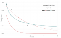
The two retention models with their best-fitting parameter compared to the data look like the following

Here is the code to generate this plot
[code lang = “R”]
library(“ggplot2”) #for plots
foo_power = function(w,t) { w[1] * t^(-w[2])} #Power curve
foo_exponential = function(w,t) {w[1] * exp(-w[2] * t)} #Exponential curve
PlotDF= data.frame(t_all=1:20, t=NA, p=NA) #DF with all x-values
PlotDF[1:20 %in% t, “t”] = obs_t #substitute data in DF
PlotDF[1:20 %in% t, “p”] = obs_p
ggplot(PlotDF, aes(x=t_all)) +
stat_function(fun = foo_power, args=list(w=R[2:3,1]), size=1, aes(color=”Power law”, linetype=”logLik”)) +
stat_function(fun = foo_power, args=list(w=R[2:3,3]), size=1, aes(color=”Power law”, linetype=”SSE”)) +
stat_function(fun = foo_exponential, args=list(w=R[2:3,2]), size=1, aes(color=”Exponential”, linetype=”logLik”)) +
stat_function(fun = foo_exponential, args=list(w=R[2:3,3]), size=1, aes(color=”Exponential”, linetype=”SSE”)) +
geom_point(aes(x=t,y=p, shape=” “), size=4, color=”white”, fill=”gray35″) +
theme_bw() +
scale_linetype_manual(“Cost functions”, values=c(“logLik”=2,”SSE”=1,”Data”=NULL)) +
scale_shape_manual(“Datapoints”, values=c(” “=21)) +
scale_color_manual(“Models”, values=c(“Exponential”=”indian red”,”Power law”=”cadet blue”)) +
scale_x_continuous(“Time [sec]”) +
scale_y_continuous(“Proportion correct”) +
theme(legend.position=c(0.8,0.8), legend.direction=”horizontal”)
ggsave(“Myung2003_illustration.png”, w=1.6*7, h=7) #save plot
[/code]
References
Myung, I. J. (2003). Tutorial on maximum likelihood estimation. Journal of Mathematical Psychology, 47, 90–100. doi:10.1016/S0022-2496(02)00028-7