
24 Dec Inter-rater reliability for unequal raters per item: Fleiss-Cuzick’s kappa
Inter rater reliability
If you want to obtain inter-rater reliability measures for dichotomous ratings, by more than two raters, but not all raters rated all items, Fleiss and Cuzick (1979) will be the referece you’ll find. For example, we asked researchers which model they consider a process model (dichotomous rating), and we asked about 60 researchers (more than two rater), of whom not everyone was familiar with every model (not all raters rated all items).
They proposed a measure between a minimum value and 1. Here is an function to calculate their kappa measure in R.
Properties
This measure, Fleiss-Cuzick’s kappa, has the following properties (see Fleiss & Cuzick, 1979).
If there is no intersubject variation in the proportion of positive judgments then there is less agreement (or more disagreement) among the judgments within than between the N subjects. In this case kappa may be seen to assume its minimum value of -1/(n-1)
If the several proportions p, vary exactly as binomial proportions with parameters n, and a common probability pbar then there is as much agreement among the judgments within the subjects as there is between the subjects. In this case, the value of kappa is equal to 0.
If each proportion pi, assumes either the values 0 or 1, then there is perfect agreement among the judgments on each subject. In this case, kappa may be seen to assume the value 1.
Note that kappa is not defined in cases of the proportions pi=0 or pi=1.
R-code implementing kappa
[code lang=”R”]# ———————————————————————————————
# Interrater-reliability for dichotomeous ratings by > 2 raters for unequal number of raters per item
# Kappa (Fleiss & Cuzick, 1979)
kappaFC = function(N, ni, xi){
# N = total number of to-be-judged items
# ni = number of judges rating the ith item
# xi = number of positive judgments on the ith item
p.i = xi / ni
qi = 1-p.i
nbar = 1/N * sum(ni) #mean number of judges
pbar = 1/(N*nbar) * sum(xi) #overall proportion positive judgments
qbar = 1-pbar
kappaFC = 1 – (sum(ni * p.i * qi) / (N * (nbar-1) * pbar * qbar))
# Minimum
minKappa = -1/(nbar-1)
# Expectation and variance
nbarH = N/sum(1/ni) #harmonic mean
eKappaFC = -1/(N * (nbar-1)) #expected value
varKappaFC = (2*(nbarH-1)) / (N*nbarH*(nbar-1)^2) + ((nbar-nbarH) * (1-4*pbar*qbar)) / (N*nbar*nbarH* (nbar-1)^2 * pbar*qbar) #variance
return(list(kappa = kappaFC, harmonicMean = nbarH, expectkappa = eKappaFC, varianceKappa = varKappaFC, minKappa = minKappa, pbar = pbar))
}[/code]
Four examples
Example 1
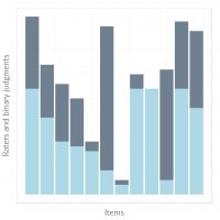
An example of 12 items judged by a differing number of judges where the colors indicate their respective ratings.
Consider the picture on the right. Imagine you have 12 items which were rated by several judges. In the plot you see the items on the x-axis (one bar per item). And on the y-axis we see how many judges rated each item (indicated by the height of the bars) and their rating (as the different colours of the bars).
If we want to know the chance-corrected agreement among these raters, we use the above mentioned kappa. Here, the inter-reater reliability equals
[latex] \kappa [/latex] = .22
This is considered a low average agreement. Values of kappa above .60 are considered high. Graphically you can see this when you look at the large proportion of half-light and half-dark bars. There are only few bars which are either mostly light or mostly dark.
This is the code to produce example 1 in R
[code lang=”R”]set.seed(5985)
N = 12
ni = sample(1:50,N)
xi = sapply(ni, sample, size=1)
kappaFC(N,ni,xi)
<[/code]
Example 2
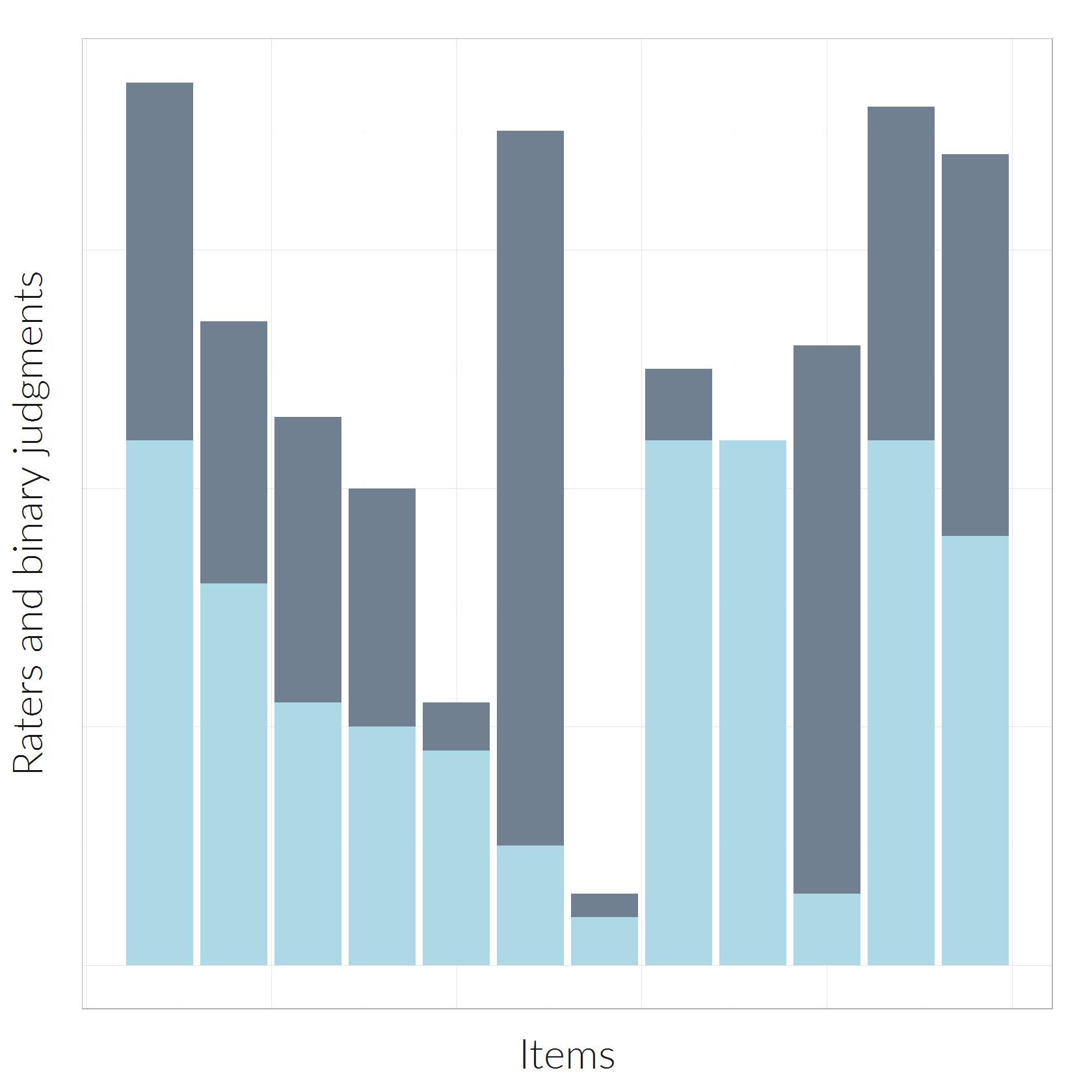
An example of 12 items where the proportion of judgments are high across all items.
Next I set the proportion to be equally high across all the twelve to-be-rated items. I simply set the number of “light” ratings by the judges such that all but one judge agreed on “light” for each of the twelve items you see on the right. Initially I expected, that kappa should be quite high, because most of the judges agree about which category the items belong to.
However, computing kappa yields
[latex] \kappa [/latex] = -0.01.
What is happening here?
Recall the properties of kappa:
If there is no intersubject variation in the proportion of positive judgments then there is less agreement (or more disagreement) among the judgments within than between the N subjects. In this case kappa may be seen to assume its minimum value of -1/(n-1)
By “intersubject variation” Fleiss and Cuzick mean the variation in ratings across items. In the plot: the variation of the colour proportions across columns. We see that the proportion of light color is constantly high for all twelve bars. Therefore, what Fleiss and Cuzick call “intersubject variation” is low. This means kappa is correctly close to -1(n-1), which, in this case is
[latex] -1(n-1) [/latex] = -0.04
.
Here’s the code to re-do example 2
[code lang=”R”]set.seed(5985)
N = 12
ni = sample(1:50,N)
xi = ni-1
kappaFC(N=N,ni=ni,xi=xi)
[/code]
Example 3
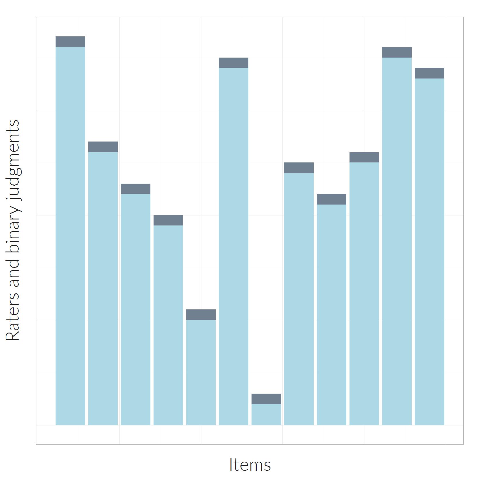
An example of 12 items where the absolute number of “light” categorizations is constant across items.
Now, let me consider raters where for each of the twelve items, the same absolute number of raters said “light” category. The corresponding pattern is illustrated in the graphic on the right. We see twelve items, one in each bar, rated by unequal numbers of judges, but the same numbe of judges (in this case: 3) agreed about the light category.
Here the kappa value computes to
[latex] \kappa [/latex] = -0.05,
which means – according to Fleiss & Cuzick – low agreement. This makes sense to me.
Here’s the code to re-do example 3
[code lang=”R”]set.seed(5985)
N = 12
ni = sample(1:50,N)
xi = rep(3,N)
kappaFC(N=N,ni=ni,xi=xi)
[/code]
Example 4

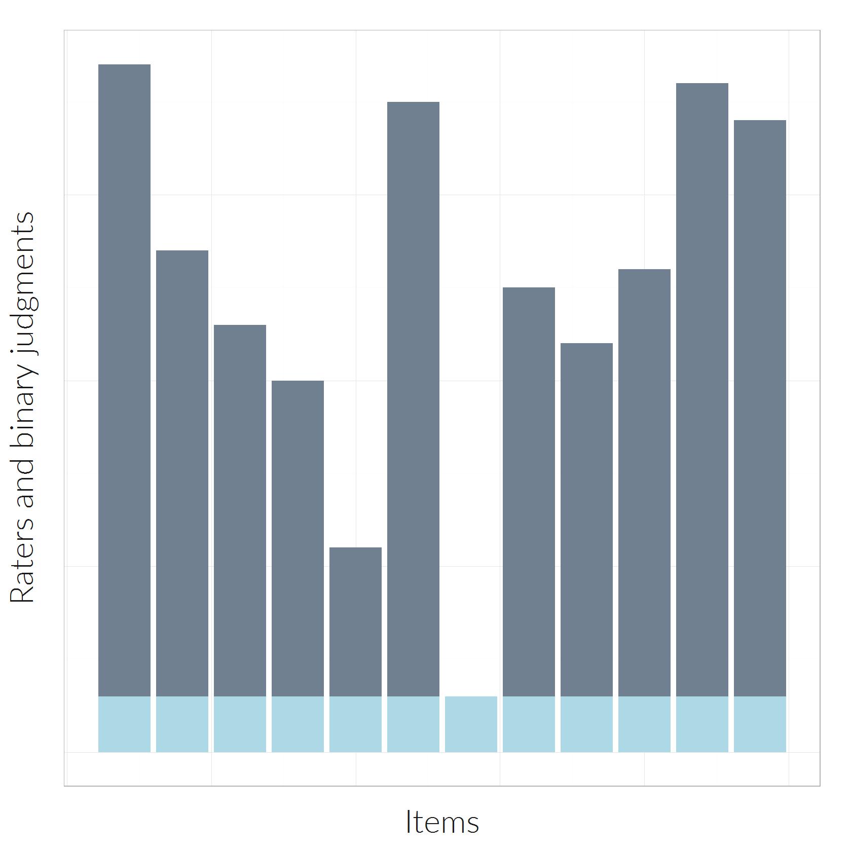
Sample data with 25 categories and binary ratings from Fleiss, Levin, & Paik (2013), p. 612
Now I will consider a sample data for which kappa turns out to be close to good agreemen. Good agreement means kappa is above .60 (see Fleiss & Cuzick). The example consists of 25 items judged by a total of 81 judges of which not all judges judged the same set of items. There were two categories from which the judges selected. We see that some judges showed complete agreement for some of the items, e.g. the first and the second column being single-colored.
Here the kappa value computes to
[latex] \kappa [/latex] = 0.54,
which means – according to Fleiss & Cuzick – moderate agreement.
Here’s the code for example 4
[code lang=”R”]set.seed(5985)
N = 25
ni = c(2,2,3,4,3,4,3,5,2,4,5,3,4,4,2,2,3,2,4,5,3,4,3,3,2)
xi = c(2,0,2,3,3,1,0,0,0,4,5,3,4,3,0,2,1,1,1,4,2,0,0,3,2)
kappaFC(N=N,ni=ni,xi=xi)
[/code]
And here is also the code to produce the figures:
[code lang=”R”]library(ggplot2) #graphics package
# Note that I use a custom R-theme, probably you want to add: + theme_bw()
ggplot(data.frame(ni=ni,xi=xi), aes(x=1:N)) +geom_bar(aes(y=ni), stat=”identity”, fill=”slategrey”) +geom_bar(aes(y=xi), stat=”identity”, fill=”lightblue”) +xlab(“Items”) +ylab(“Raters and binary judgments”) +theme(axis.text=element_blank(), axis.ticks=element_blank())
[/code]
Reference
Fleiss, J. L., & Cuzick, J. (1979). The reliability of dichotomous judgments: Unequal numbers of judges per subject. Applied Psychological Measurement, 3(4), 537–542. doi:10.1177/014662167900300410
Fleiss, J. L., Levin, B., & Paik, M. C. (2013). Statistical methods for rates and proportions. John Wiley & Sons.